LiDAR 3D
The LiDAR 3D widget renders, in a real-time three-dimensional scene, every entity a LiDAR sensor is tracking: people, vehicles and any other body detected within its field of view.
Unlike a camera, a LiDAR sensor does not deliver an image but a point cloud, which the driver turns into objects with position, size, speed and confidence. The widget takes those objects and draws them as boxes inside a navigable scene, on which you can also overlay the configured zones and a 3D model of the real environment (an industrial plant, a maneuvering yard, a building).
This makes it possible to answer at a glance questions a camera does not answer well: how many people are in the yard right now?, did anyone step into the crane's swing radius?, how fast are the forklifts moving?
Prerequisites
Before adding the widget you need:
| Requirement | Detail |
|---|---|
| Driver installed | The LiDAR sensor driver must be installed and running on the site. |
| Device registered | The sensor must exist as a device, for example QUANERGY SIMULATED. |
| A LiDAR-type sensor object | The device must contain an object of type sensor whose sensor_type property is lidar. Only those objects appear in the widget's selector. |
| User permission | Your user needs the dashboard:canSeeSensorWidget permission. Without it, the widget does not appear in the catalog. |
INFO The tracked entities are not objects you create by hand: the driver publishes them as Relative Tracker objects associated with the sensor. Zones are Relative Zone objects anchored to that same sensor.
Step 1: Add the widget to the dashboard
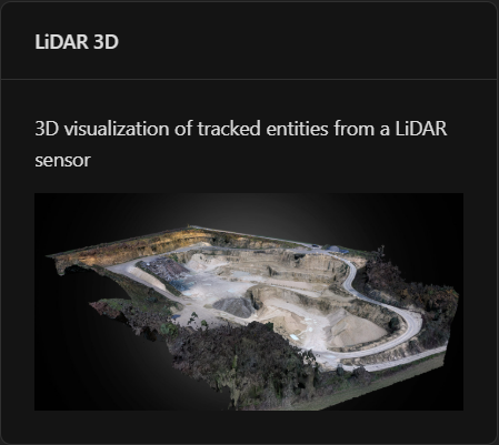
From your dashboard, press Add and pick the LiDAR 3D card from the widget catalog.
Step 2: Select the sensor
The widget asks you to choose the data source. Open Select a LiDAR sensor and pick the corresponding sensor.

The dropdown lists only the LiDAR sensors available in the system. In a test environment, for instance, the simulated sensor shows up as Quanergy Qortex Device localhost.
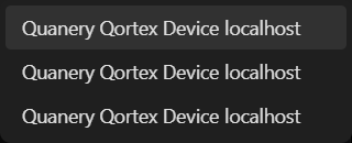
Confirm with Select object. The 3D scene starts rendering right away with the entities the sensor is reporting at that moment.
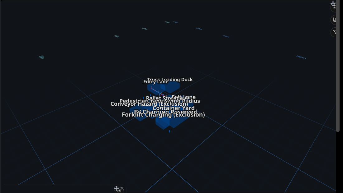
At first you will only see the reference grid (with distance marks every 50 m), the configured zones and the moving entities. The 3D environment is loaded later, in Step 4.
Step 3: Navigate the scene
The scene is operated with the mouse:
| Action | Result |
|---|---|
| Left click + drag | Orbits the camera around the scene. |
| Mouse wheel | Zooms in or out. |
| Right click + drag | Moves the camera sideways (pan). |
| Click on an entity | Selects it: it is highlighted in cyan and the camera flies toward it to frame it. |
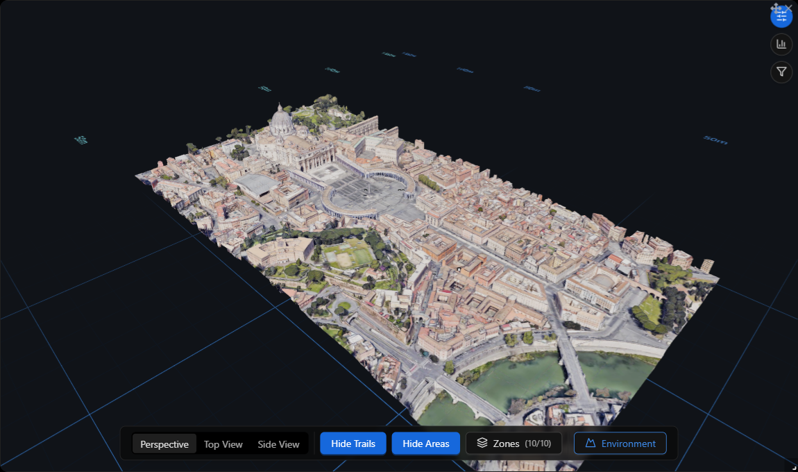
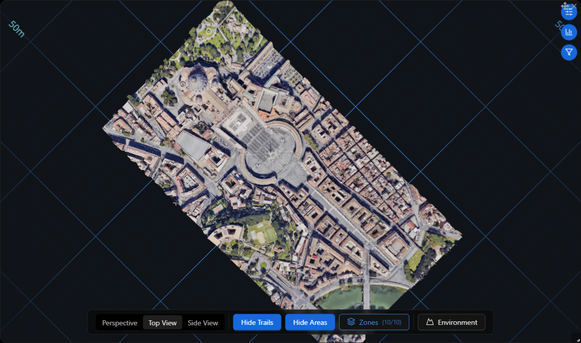
To open the scene controls, use the 3D Controls button (sliders icon), the first of the three circular buttons in the widget's upper-right corner. A bar then appears at the bottom:

Camera modes
The first three buttons set the viewing angle:
- Perspective — perspective view, the default mode. Useful for understanding volumes and heights.
- Top View — overhead view, from above. It is the most practical one for reading positions, distances and zone occupancy.
- Side View — side view. It helps verify heights and tell apart entities that overlap in the overhead view.
Trails
The button toggles between Hide Trails and Show Trails. Trails are the lines that trace each entity's recent path; they are active by default and keep up to the last 50 points of every trajectory. Their color follows the entity's status.
They are especially useful for reconstructing where someone went in the last few seconds, or for spotting abnormal circulation patterns.
Areas (zones)
The button toggles between Hide Areas and Show Areas, and shows or hides all zones at once. For individual control, use the Zones button.
Step 4: Load the 3D environment
By default the scene is an empty space with a grid. To give it context you can load a three-dimensional model of the actual facility. Press Environment in the controls bar.
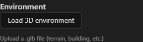
Press Load 3D environment and select a file. The panel accepts models in .glb or .gltf format, with a maximum size of 100 MB.
Once loaded, the panel shows the file name and four fields to align the model with the sensor's coordinate system:
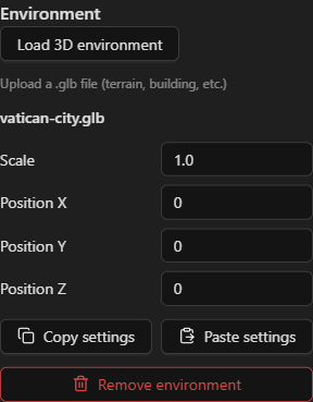
| Field | Purpose |
|---|---|
| Scale | The model's scale factor. Adjust it until the model's dimensions match the grid's distance marks. |
| Position X / Y / Z | Shift the model along each axis so its origin matches the sensor's. |
TIP Align the model using Top View and the grid's distance labels as a reference. It is much faster than doing it in perspective.
The Copy settings button copies only the scale and the position to the clipboard —never the model file— and Paste settings applies them to another sensor. It is the practical way to replicate an already fine-tuned calibration across several sensors that share the same environment model.
Remove environment deletes the model and resets the scale to 1 and the position to (0, 0, 0).
NOTE The environment configuration is saved per sensor and on the server, not in your browser. Loading a model uploads it immediately; scale and position changes are saved automatically about half a second after you stop typing. Any user who opens that sensor will see the same, already calibrated environment.
Step 5: Control zone visibility
Zones are polygons configured over the sensor's coverage area: entry and exit lanes, pedestrian walkways, machinery swing radii, loading areas. The widget draws them as translucent volumes with the zone name floating above them.
The Zones button in the controls bar shows a (visible/total) counter and opens the full list:
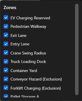
Each checkbox shows or hides that zone individually in the scene. Hiding a zone is purely visual: it is still evaluated and the automations associated with it are unaffected.
INFO The name you see is exactly the one configured on the Relative Zone object in the system. Suffixes such as
(Exclusion)in the example above are part of the name given by whoever configured the zone; the widget neither interprets them nor treats them in any special way.
Step 6: Filter the entities
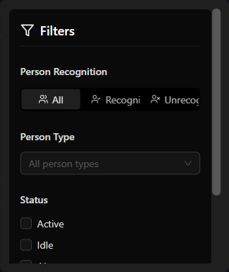
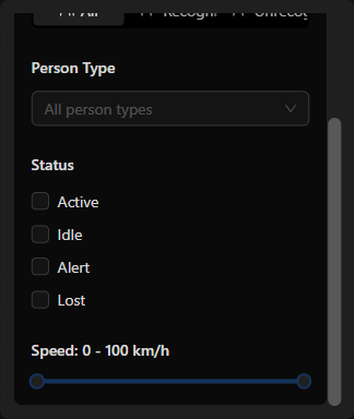
The third circular button, Filters (funnel icon), opens the filters panel. Filters affect both what is drawn in the scene and the values in the KPIs panel.
Person Recognition
Segments entities according to whether they could be matched to a person registered in the system:
- All — every entity, recognized or not.
- Recognized — only entities linked to a known person.
- Unrecognized — only entities with no associated person.
Recognized entities are drawn with a floating circular marker above the box, showing the person's photo and a ring in the color of their person type.
Person Type
Restricts the view to one or more person types (employee, visitor, contractor…). Each option is shown with the color dot assigned to that type. If you choose none, no restriction is applied.
This control is disabled when the previous filter is set to Unrecognized, because an entity with no associated person has no person type either.
Status
Checkboxes for an entity's four possible statuses: Active, Idle, Alert and Lost. If you check none, all of them are shown.
The status also determines the color of the box in the scene:
| Status | Entity color |
|---|---|
| Alert | Red |
| Idle | Amber |
| Selected | Cyan |
| Everything else | Blue, or the entity's own color |
Speed
A range slider, in steps of 5, that limits the view to entities whose speed falls within the chosen interval. As long as the range is complete (0 - 100), no filter is applied.
KPIs panel
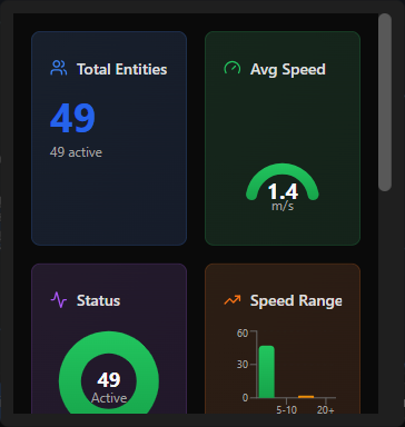
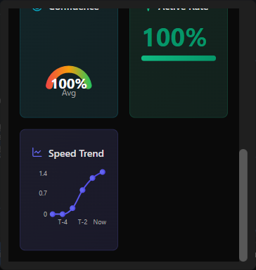
The middle button, KPIs (bar chart icon), summarizes the aggregate status of the entities that pass the active filters in seven cards.
| Card | What it shows |
|---|---|
| Total Entities | Number of visible entities, and below it how many of them are active. |
| Avg Speed | Average speed of all visible entities, in a semicircular gauge. |
| Status | Distribution of entities by status, as a doughnut chart. |
| Speed Range | How many entities fall in each speed band: 0-5, 5-10, 10-20 and 20+. |
| Confidence | Average confidence with which the sensor detects the entities, as a percentage. Low confidence is also reflected in the scene: the entity's box is drawn more transparent. |
| Active Rate | Percentage of visible entities that are in the active status. |
| Speed Trend | A visual reading of the average speed, where the Now point corresponds to the live value. |
NOTE The average speed is expressed in m/s on the Avg Speed card, while the filters panel slider and the entity list label it in km/h. Both operate on the same value delivered by the sensor.
How an entity is represented
Each tracked entity is drawn as a three-dimensional box whose dimensions come from the size estimated by the sensor. Its transparency reflects the confidence of the detection: the more translucent it is, the less certain the sensor is about what it sees.
Two elements may appear on top of that box:
- The person marker, if the entity was matched to someone registered. It is a disc with the photo and a ring in the color of the person type, always facing the camera.
- The trail, if trails are active, tracing the recent path.
When you click an entity, it is highlighted in cyan and the camera automatically moves closer to frame it, keeping the current viewing angle.
The data behind each entity —position, size, speed, heading and confidence— comes from the state properties of the Relative Tracker object published by the driver. See Relative Tracker and Relative Zone for the detail of each property.
Best practices
- Use Top View to operate and Perspective to present. The overhead view is the one that lets you read real distances without perspective distortion.
- Calibrate the environment once and replicate it. Adjust scale and position on one sensor, and use Copy settings / Paste settings on the rest.
- Hide the zones you are not watching. With many overlapping zones, the floating labels pile up and the scene becomes hard to read.
- Back the widget with automations. The visualization is there to understand what is happening; to react to an entry into an exclusion zone, create a rule on the state of the corresponding Relative Zone object.